The Lab · instrument 09/12 · interactive

Grow an embedding space

Real distributional embeddings — co-occurrence counts, PPMI rows as vectors, an eigensolve for the picture — trained live on whatever you type, with neighbors computed in the full space and an honest 2D shadow of it.

What's real here

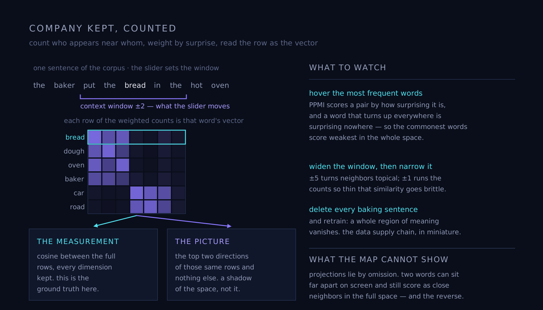
This is the count-based recipe that preceded — and still explains — neural embeddings: count which words appear near which (your context-window slider), weight the counts by how surprising they are (positive pointwise mutual information), and read each word's row of that matrix as its vector. The 2D scatter is the top two directions of a factorization of those rows; the neighbor list when you hover is cosine similarity between the full rows. Word2vec and its descendants learn a compressed version of almost exactly this signal — "you shall know a word by the company it keeps," made arithmetic.

Where to push

The default corpus mixes pets, cars, and baking; hover cat and find dog, hover bread and find dough — no dictionary was consulted, only company kept. Now hover the, then a: the corpus's most frequent words have the weakest neighbor scores in the whole space, because PPMI scores a pair by how surprising the pairing is, and a word that turns up everywhere is surprising nowhere — real pipelines fight exactly this with subsampling and context weighting. Widen the window to ±5 and neighbors turn topical (bread pulls in oven and baker); narrow it to ±1 and the counts run so thin that similarities go brittle — a live preview of why these pipelines want millions of tokens, not a paragraph. Then delete every baking sentence and retrain: watch a whole region of meaning vanish, which is the data supply chain demonstrated in miniature.

Failure mode

Trusting the picture over the space. The scatter is a projection — two dimensions kept out of dozens — and projections lie by omission: two words can sit far apart on screen yet score as close neighbors in the full space, and the reverse. That's why the neighbor list, not the map, is the ground truth here — and why the same skepticism applies to every t-SNE and UMAP plot in every embedding demo you'll ever be shown. Pretty maps are summaries; similarity scores are the measurements.